Breast Cancer problem.
This is a problem that I have trid to solve using just the old tidymodels package and got stuck so here is the new implementation using the amazing tune and workflows packages
Setting up Rmarkdown
root.dir =
Loading Libraries
library(tidyverse)## -- Attaching packages ---------------------------------------------------------------------------------------------------------------------------------------------- tidyverse 1.3.0 --## <U+2713> ggplot2 3.2.1 <U+2713> purrr 0.3.3
## <U+2713> tibble 2.1.3 <U+2713> dplyr 0.8.3
## <U+2713> tidyr 1.0.0 <U+2713> stringr 1.4.0
## <U+2713> readr 1.3.1 <U+2713> forcats 0.4.0## -- Conflicts ------------------------------------------------------------------------------------------------------------------------------------------------- tidyverse_conflicts() --
## x dplyr::filter() masks stats::filter()
## x dplyr::lag() masks stats::lag()library(tidymodels)## Registered S3 method overwritten by 'xts':
## method from
## as.zoo.xts zoo## -- Attaching packages --------------------------------------------------------------------------------------------------------------------------------------------- tidymodels 0.0.3 --## <U+2713> broom 0.5.3 <U+2713> recipes 0.1.8
## <U+2713> dials 0.0.4 <U+2713> rsample 0.0.5
## <U+2713> infer 0.5.1 <U+2713> yardstick 0.0.4
## <U+2713> parsnip 0.0.4## -- Conflicts ------------------------------------------------------------------------------------------------------------------------------------------------ tidymodels_conflicts() --
## x scales::discard() masks purrr::discard()
## x dplyr::filter() masks stats::filter()
## x recipes::fixed() masks stringr::fixed()
## x dplyr::lag() masks stats::lag()
## x dials::margin() masks ggplot2::margin()
## x yardstick::spec() masks readr::spec()
## x recipes::step() masks stats::step()
## x recipes::yj_trans() masks scales::yj_trans()library(janitor)##
## Attaching package: 'janitor'## The following objects are masked from 'package:stats':
##
## chisq.test, fisher.testlibrary(skimr)
library(DataExplorer)Loading Libraries: 3.65 sec elapsed
Getting Data
Got the dataset with headers on kaggle link, there is also a cool explanation about the problem there.
df <- read_csv("breast_cancer.csv")## Warning: Missing column names filled in: 'X33' [33]## Parsed with column specification:
## cols(
## .default = col_double(),
## diagnosis = col_character(),
## X33 = col_character()
## )## See spec(...) for full column specifications.## Warning: 569 parsing failures.
## row col expected actual file
## 1 -- 33 columns 32 columns 'breast_cancer.csv'
## 2 -- 33 columns 32 columns 'breast_cancer.csv'
## 3 -- 33 columns 32 columns 'breast_cancer.csv'
## 4 -- 33 columns 32 columns 'breast_cancer.csv'
## 5 -- 33 columns 32 columns 'breast_cancer.csv'
## ... ... .......... .......... ...................
## See problems(...) for more details.Set Chunk: 0.16 sec elapsed
There is a strange extra column named X33 dealing with that using janitor package
df <- df %>%
  janitor::remove_empty_cols()
## Warning: 'janitor::remove_empty_cols' is deprecated.
## Use 'remove_empty("cols")' instead.
## See help("Deprecated")Cleaning Data: 0.01 sec elapsed
Visualizing the data using DataExplorer and Skimr
Skimr is a fast way to get info on your data even though the hist plot fails on my blog :(
df %>%
skimr::skim()| Name | Piped data |
| Number of rows | 569 |
| Number of columns | 32 |
| _______________________ | |
| Column type frequency: | |
| character | 1 |
| numeric | 31 |
| ________________________ | |
| Group variables | None |
Variable type: character
| skim_variable | n_missing | complete_rate | min | max | empty | n_unique | whitespace |
|---|---|---|---|---|---|---|---|
| diagnosis | 0 | 1 | 1 | 1 | 0 | 2 | 0 |
Variable type: numeric
| skim_variable | n_missing | complete_rate | mean | sd | p0 | p25 | p50 | p75 | p100 | hist |
|---|---|---|---|---|---|---|---|---|---|---|
| id | 0 | 1 | 30371831.43 | 125020585.61 | 8670.00 | 869218.00 | 906024.00 | 8813129.00 | 911320502.00 | ▇▁▁▁▁ |
| radius_mean | 0 | 1 | 14.13 | 3.52 | 6.98 | 11.70 | 13.37 | 15.78 | 28.11 | ▂▇▃▁▁ |
| texture_mean | 0 | 1 | 19.29 | 4.30 | 9.71 | 16.17 | 18.84 | 21.80 | 39.28 | ▃▇▃▁▁ |
| perimeter_mean | 0 | 1 | 91.97 | 24.30 | 43.79 | 75.17 | 86.24 | 104.10 | 188.50 | ▃▇▃▁▁ |
| area_mean | 0 | 1 | 654.89 | 351.91 | 143.50 | 420.30 | 551.10 | 782.70 | 2501.00 | ▇▃▂▁▁ |
| smoothness_mean | 0 | 1 | 0.10 | 0.01 | 0.05 | 0.09 | 0.10 | 0.11 | 0.16 | ▁▇▇▁▁ |
| compactness_mean | 0 | 1 | 0.10 | 0.05 | 0.02 | 0.06 | 0.09 | 0.13 | 0.35 | ▇▇▂▁▁ |
| concavity_mean | 0 | 1 | 0.09 | 0.08 | 0.00 | 0.03 | 0.06 | 0.13 | 0.43 | ▇▃▂▁▁ |
| concave points_mean | 0 | 1 | 0.05 | 0.04 | 0.00 | 0.02 | 0.03 | 0.07 | 0.20 | ▇▃▂▁▁ |
| symmetry_mean | 0 | 1 | 0.18 | 0.03 | 0.11 | 0.16 | 0.18 | 0.20 | 0.30 | ▁▇▅▁▁ |
| fractal_dimension_mean | 0 | 1 | 0.06 | 0.01 | 0.05 | 0.06 | 0.06 | 0.07 | 0.10 | ▆▇▂▁▁ |
| radius_se | 0 | 1 | 0.41 | 0.28 | 0.11 | 0.23 | 0.32 | 0.48 | 2.87 | ▇▁▁▁▁ |
| texture_se | 0 | 1 | 1.22 | 0.55 | 0.36 | 0.83 | 1.11 | 1.47 | 4.88 | ▇▅▁▁▁ |
| perimeter_se | 0 | 1 | 2.87 | 2.02 | 0.76 | 1.61 | 2.29 | 3.36 | 21.98 | ▇▁▁▁▁ |
| area_se | 0 | 1 | 40.34 | 45.49 | 6.80 | 17.85 | 24.53 | 45.19 | 542.20 | ▇▁▁▁▁ |
| smoothness_se | 0 | 1 | 0.01 | 0.00 | 0.00 | 0.01 | 0.01 | 0.01 | 0.03 | ▇▃▁▁▁ |
| compactness_se | 0 | 1 | 0.03 | 0.02 | 0.00 | 0.01 | 0.02 | 0.03 | 0.14 | ▇▃▁▁▁ |
| concavity_se | 0 | 1 | 0.03 | 0.03 | 0.00 | 0.02 | 0.03 | 0.04 | 0.40 | ▇▁▁▁▁ |
| concave points_se | 0 | 1 | 0.01 | 0.01 | 0.00 | 0.01 | 0.01 | 0.01 | 0.05 | ▇▇▁▁▁ |
| symmetry_se | 0 | 1 | 0.02 | 0.01 | 0.01 | 0.02 | 0.02 | 0.02 | 0.08 | ▇▃▁▁▁ |
| fractal_dimension_se | 0 | 1 | 0.00 | 0.00 | 0.00 | 0.00 | 0.00 | 0.00 | 0.03 | ▇▁▁▁▁ |
| radius_worst | 0 | 1 | 16.27 | 4.83 | 7.93 | 13.01 | 14.97 | 18.79 | 36.04 | ▆▇▃▁▁ |
| texture_worst | 0 | 1 | 25.68 | 6.15 | 12.02 | 21.08 | 25.41 | 29.72 | 49.54 | ▃▇▆▁▁ |
| perimeter_worst | 0 | 1 | 107.26 | 33.60 | 50.41 | 84.11 | 97.66 | 125.40 | 251.20 | ▇▇▃▁▁ |
| area_worst | 0 | 1 | 880.58 | 569.36 | 185.20 | 515.30 | 686.50 | 1084.00 | 4254.00 | ▇▂▁▁▁ |
| smoothness_worst | 0 | 1 | 0.13 | 0.02 | 0.07 | 0.12 | 0.13 | 0.15 | 0.22 | ▂▇▇▂▁ |
| compactness_worst | 0 | 1 | 0.25 | 0.16 | 0.03 | 0.15 | 0.21 | 0.34 | 1.06 | ▇▅▁▁▁ |
| concavity_worst | 0 | 1 | 0.27 | 0.21 | 0.00 | 0.11 | 0.23 | 0.38 | 1.25 | ▇▅▂▁▁ |
| concave points_worst | 0 | 1 | 0.11 | 0.07 | 0.00 | 0.06 | 0.10 | 0.16 | 0.29 | ▅▇▅▃▁ |
| symmetry_worst | 0 | 1 | 0.29 | 0.06 | 0.16 | 0.25 | 0.28 | 0.32 | 0.66 | ▅▇▁▁▁ |
| fractal_dimension_worst | 0 | 1 | 0.08 | 0.02 | 0.06 | 0.07 | 0.08 | 0.09 | 0.21 | ▇▃▁▁▁ |
Skimr: 0.15 sec elapsed
Data Explorer
Is a imho a prettier option with individual cool plots and a super powerfull(but slow) report creation tool when working outside of an Rmarkdownm document
df %>%
  DataExplorer::plot_intro()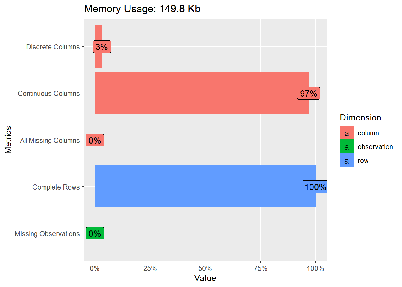
df %>%
  DataExplorer::plot_bar()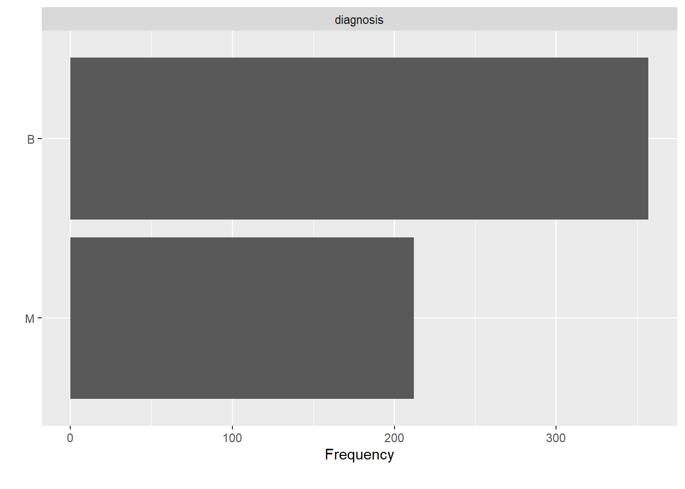
df %>%
DataExplorer::plot_correlation()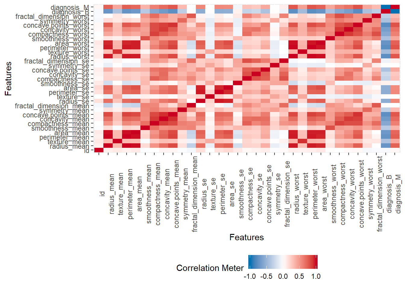 Data Explorer individual plots: 1.05 sec elapsed
There are much more amaziong tools such as the ggforce package , but I hope you get the gist of the exploration stage.
Modeling
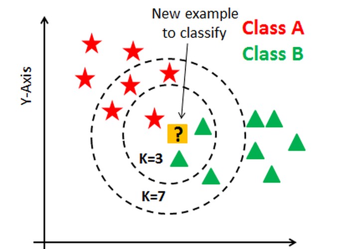
For now I am going to focus on the tools provided by the tidymodels packages and the KNN, in the future I may come back to add more models and probably to play around the DALEX package a little bit.
Just to remember M is Malignant and B is Benign, we are trying to correcly classify our patients, I am going to ignore the id Varible since it should not be reliaded upon to generate predictions(Even though it may capture some interesting effects such as better screening for patients on the latter id’s).
Train Test Split
Usually we split our data into training and test data to ensure a fair evaluation of the models or parameters being tested(hoping to avoid overfitting).
The workflow for the tidymodels is that we first split our data.
df_split <- df %>%
  rsample::initial_split(prop = 0.8)
Initial Split: 0 sec elapsed
df_training <- df_split %>% training()
df_testing <- df_split %>% testing()
Train test split: 0.02 sec elapsed
Then we model on our Training Data
Recipes
Recipes are used to preprocess our data, the main mistake here is using the whole data set.
The recipe package helps us with this process.
For those not familiarized with the formula notation I am fitting the model on all variables except the id variable.
I am than Normalizing my data since the KNN alghoritm is sensible to the scale of the variables being used, I am also excluding variables with high absolute correlation amongst themselves.
Recipes are easy to read and can be quite complex
df_recipe <- training(df_split) %>%
  recipe(diagnosis ~ .) %>%
  step_rm(id) %>%
  step_center(all_predictors()) %>%
  step_scale(all_predictors(),all_numeric()) %>%
  step_corr(all_predictors())
recipes: 0 sec elapsed
We could then create our train and test data frames by baking our recipe and juicing our recipe
# df_testing <- df_recipe %>%
#   bake(testing(df_split))
# df_testing
#df_training <- juice(df_recipe)
unnamed-chunk-1: 0 sec elapsed
But I am going for a Bayes search approch
Cross Validation and Bayes Search
Cross Validation
We further divide our data frame into folds in order to improve our certainty that the ideal number of neighbours is right.
cv_splits <- df_testing %>% vfold_cv(v = 5)cvfold split: 0.02 sec elapsed
Using the new tune package currently on github
library(tune)
knn_mod <-
  nearest_neighbor(neighbors = tune(), weight_func = tune()) %>%
  set_engine("kknn") %>%
  set_mode("classification")
unnamed-chunk-2: 0.05 sec elapsed
Combining everything so far in the new package workflow
library(workflows)
knn_wflow <-
  workflow() %>%
  add_model(knn_mod) %>%
  add_recipe(df_recipe)
unnamed-chunk-3: 0.04 sec elapsed
Limiting our search
knn_param <-
  knn_wflow %>%
  parameters() %>%
    update(
    neighbors = neighbors(c(3, 50)),
    weight_func = weight_func(values = c("rectangular", "inv", "gaussian", "triangular"))
  )
unnamed-chunk-4: 0.03 sec elapsed
Searching for the best model
I used 5 iterations as the limit for the process because of printing reasons.
Keep in mind that mtune will maximize just the first metric from the package yardstick
ctrl <- control_bayes(verbose = TRUE,no_improve = 5)
set.seed(42)
knn_search <- tune_bayes(knn_wflow,
                         resamples = cv_splits,
                         initial = 5,
                         iter = 20,
                         param_info = knn_param,
                         control = ctrl,
                         metrics = metric_set(roc_auc,accuracy))
## ## > Generating a set of 5 initial parameter results## v Initialization complete## ## Optimizing roc_auc using the expected improvement## ## -- Iteration 1 ------------------------------------------------------------------------------------------------------------------------------------------------------------------------## ## i Current best: roc_auc=0.9706 (@iter 0)## i Gaussian process model## v Gaussian process model## i Generating 139 candidates## i Predicted candidates## i neighbors=31, weight_func=inv## i Estimating performance## v Estimating performance## <U+24E7> Newest results: roc_auc=0.969 (+/-0.013)## ## -- Iteration 2 ------------------------------------------------------------------------------------------------------------------------------------------------------------------------## ## i Current best: roc_auc=0.9706 (@iter 0)## i Gaussian process model## v Gaussian process model## i Generating 138 candidates## i Predicted candidates## i neighbors=3, weight_func=rectangular## i Estimating performance## v Estimating performance## <U+24E7> Newest results: roc_auc=0.9538 (+/-0.0208)## ## -- Iteration 3 ------------------------------------------------------------------------------------------------------------------------------------------------------------------------## ## i Current best: roc_auc=0.9706 (@iter 0)## i Gaussian process model## v Gaussian process model## i Generating 137 candidates## i Predicted candidates## i neighbors=50, weight_func=rectangular## i Estimating performance## v Estimating performance## <U+24E7> Newest results: roc_auc=0.9432 (+/-0.0214)## ## -- Iteration 4 ------------------------------------------------------------------------------------------------------------------------------------------------------------------------## ## i Current best: roc_auc=0.9706 (@iter 0)## i Gaussian process model## v Gaussian process model## i Generating 136 candidates## i Predicted candidates## i neighbors=15, weight_func=rectangular## i Estimating performance## v Estimating performance## <U+24E7> Newest results: roc_auc=0.9676 (+/-0.0184)## ## -- Iteration 5 ------------------------------------------------------------------------------------------------------------------------------------------------------------------------## ## i Current best: roc_auc=0.9706 (@iter 0)## i Gaussian process model## v Gaussian process model## i Generating 135 candidates## i Predicted candidates## i neighbors=3, weight_func=gaussian## i Estimating performance## v Estimating performance## <U+24E7> Newest results: roc_auc=0.9562 (+/-0.0205)## ! No improvement for 5 iterations; returning current results.Bayes Search: 26.38 sec elapsed
Visualizing our search
autoplot(knn_search, type = "performance", metric = "accuracy")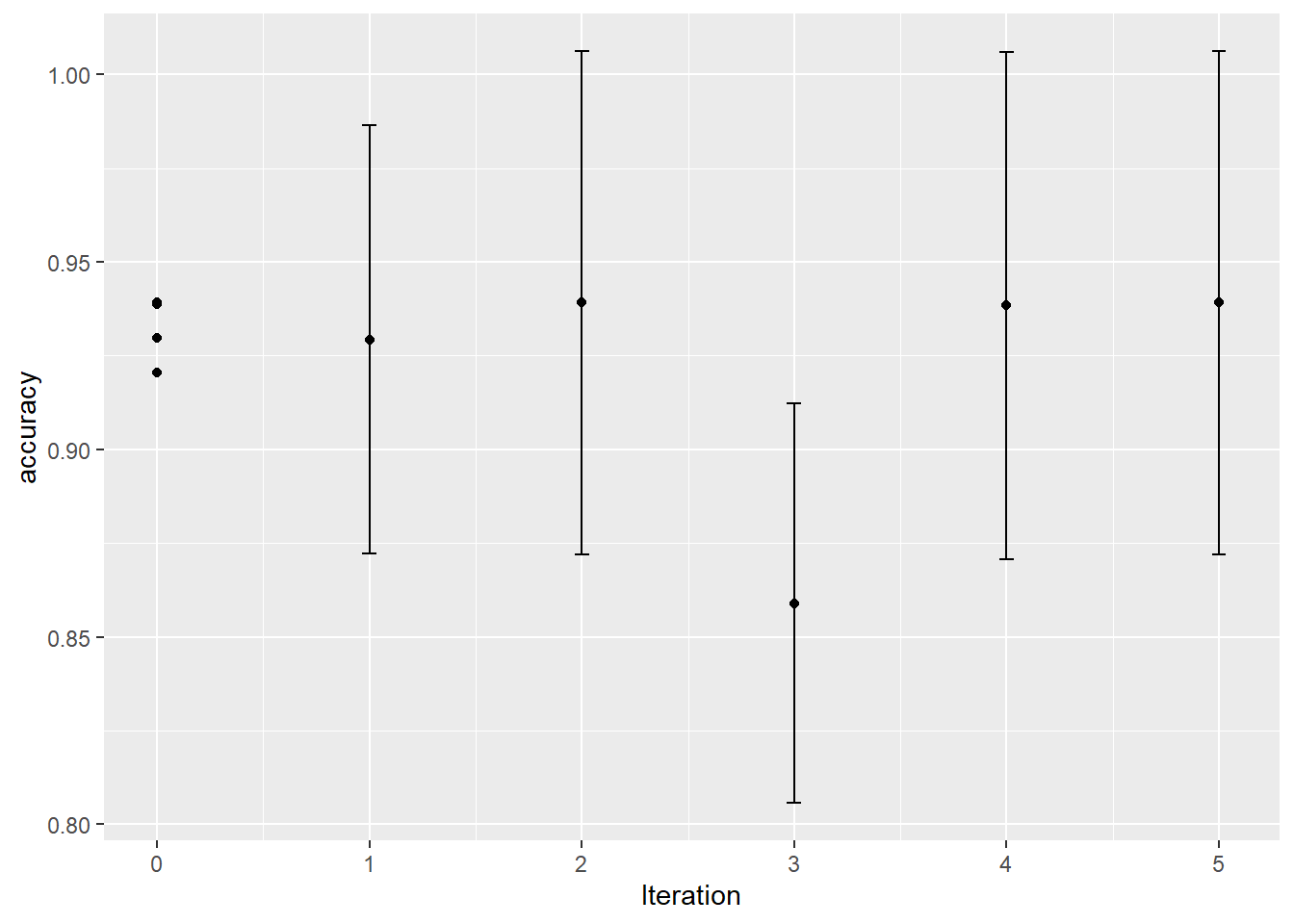 unnamed-chunk-5: 0.16 sec elapsed
autoplot(knn_search, type = "performance", metric = "roc_auc")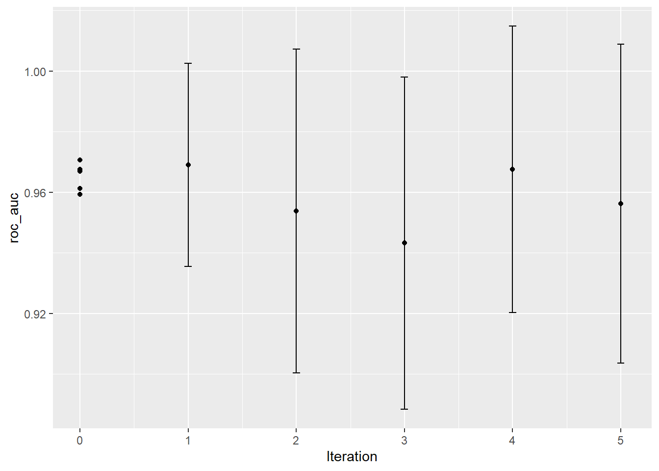 unnamed-chunk-6: 0.2 sec elapsed
Seing the best result
collect_metrics(knn_search) %>%
  dplyr::filter(.metric == "accuracy") %>%
  arrange(mean %>% desc)
## # A tibble: 10 x 8
## neighbors weight_func .iter .metric .estimator mean n std_err
## <int> <chr> <dbl> <chr> <chr> <dbl> <int> <dbl>
## 1 3 gaussian 5 accuracy binary 0.939 5 0.0261
## 2 3 rectangular 2 accuracy binary 0.939 5 0.0261
## 3 5 inv 0 accuracy binary 0.939 5 0.0295
## 4 13 inv 0 accuracy binary 0.939 5 0.0221
## 5 42 gaussian 0 accuracy binary 0.939 5 0.0294
## 6 15 rectangular 4 accuracy binary 0.938 5 0.0263
## 7 33 inv 0 accuracy binary 0.930 5 0.0259
## 8 31 inv 1 accuracy binary 0.929 5 0.0222
## 9 27 rectangular 0 accuracy binary 0.921 5 0.0253
## 10 50 rectangular 3 accuracy binary 0.859 5 0.0207unnamed-chunk-7: 0.03 sec elapsed
collect_metrics(knn_search) %>%
  dplyr::filter(.metric == "roc_auc") %>%
  arrange(mean %>% desc)
## # A tibble: 10 x 8
## neighbors weight_func .iter .metric .estimator mean n std_err
## <int> <chr> <dbl> <chr> <chr> <dbl> <int> <dbl>
## 1 33 inv 0 roc_auc binary 0.971 5 0.0165
## 2 31 inv 1 roc_auc binary 0.969 5 0.0130
## 3 42 gaussian 0 roc_auc binary 0.968 5 0.0182
## 4 15 rectangular 4 roc_auc binary 0.968 5 0.0184
## 5 13 inv 0 roc_auc binary 0.967 5 0.0203
## 6 27 rectangular 0 roc_auc binary 0.961 5 0.0168
## 7 5 inv 0 roc_auc binary 0.959 5 0.0182
## 8 3 gaussian 5 roc_auc binary 0.956 5 0.0205
## 9 3 rectangular 2 roc_auc binary 0.954 5 0.0208
## 10 50 rectangular 3 roc_auc binary 0.943 5 0.0214unnamed-chunk-8: 0.03 sec elapsed
Extracting the best model
best_metrics <- collect_metrics(knn_search) %>%
  dplyr::filter(.metric == "roc_auc") %>%
  arrange(mean %>% desc) %>%
  head(1) %>%
  select(neighbors,weight_func) %>%
  as.list()
unnamed-chunk-9: 0.01 sec elapsed
Creating production model
production_knn <-
  nearest_neighbor(neighbors = best_metrics$neighbors,weight_func = best_metrics$weight_func) %>%
  set_engine("kknn") %>%
  set_mode("classification")
unnamed-chunk-10: 0 sec elapsed
Creating production wflow
production_wflow <-   workflow() %>%
  add_model(production_knn) %>%
  add_recipe(df_recipe)
unnamed-chunk-11: 0 sec elapsed
Finally applying testing production model
fit_prod <- fit(production_wflow,df_training)Fitting production: 0.28 sec elapsed
Metrics
fit_prod %>% predict(df_testing) %>%
  bind_cols(df_testing %>% transmute(diagnosis = diagnosis %>% as.factor())) %>%
  yardstick::metrics(truth = diagnosis,estimate = .pred_class)
## # A tibble: 2 x 3
## .metric .estimator .estimate
## <chr> <chr> <dbl>
## 1 accuracy binary 0.965
## 2 kap binary 0.926Calculating metrics: 0.03 sec elapsed
predict(fit_prod,df_testing,type = 'prob') %>%
  bind_cols(df_testing %>% transmute(diagnosis = diagnosis %>% as.factor())) %>%
  yardstick::roc_auc(truth = diagnosis,.pred_B)
## # A tibble: 1 x 3
## .metric .estimator .estimate
## <chr> <chr> <dbl>
## 1 roc_auc binary 0.989Calculating metrics auc: 0.04 sec elapsed
Another visualization
knn_naive <-
  nearest_neighbor(neighbors = tune()) %>%
  set_engine("kknn") %>%
  set_mode("classification")
unnamed-chunk-12: 0 sec elapsed
Combining everything so far in the new package workflow
knn_wflow_naive <-
  workflow() %>%
  add_model(knn_naive) %>%
  add_recipe(df_recipe)
unnamed-chunk-13: 0 sec elapsed
knn_naive_param <-
  knn_wflow %>%
  parameters() %>%
    update(
    neighbors = neighbors(c(10, 50))
  )
unnamed-chunk-14: 0.02 sec elapsed
One advantage of the naive search is that it is easy to parallelize
all_cores <- parallel::detectCores(logical = FALSE)

library(doParallel)
## Loading required package: foreach##
## Attaching package: 'foreach'## The following objects are masked from 'package:purrr':
##
## accumulate, when## Loading required package: iterators## Loading required package: parallelcl <- makePSOCKcluster(all_cores)
registerDoParallel(cl)set up parallel: 1.29 sec elapsed
ctrl <- control_grid(verbose = FALSE)
set.seed(42)
naive_search <- tune_grid(knn_wflow_naive,
                         resamples = cv_splits,
                         param_info = knn_naive_param,
                         control = ctrl,
                         grid = 50,
                         metrics = metric_set(roc_auc,accuracy))
naive grid search: 6.31 sec elapsed
best_naive_metrics <- collect_metrics(naive_search) %>%
  dplyr::filter(.metric == "roc_auc") %>%
  arrange(mean %>% desc)
DT::datatable(best_naive_metrics,options = list(pageLength = 5, scrollX=T))p <- best_naive_metrics %>%
ggplot() +
aes(neighbors,mean) +
geom_point() +
ylim(.95,1)
p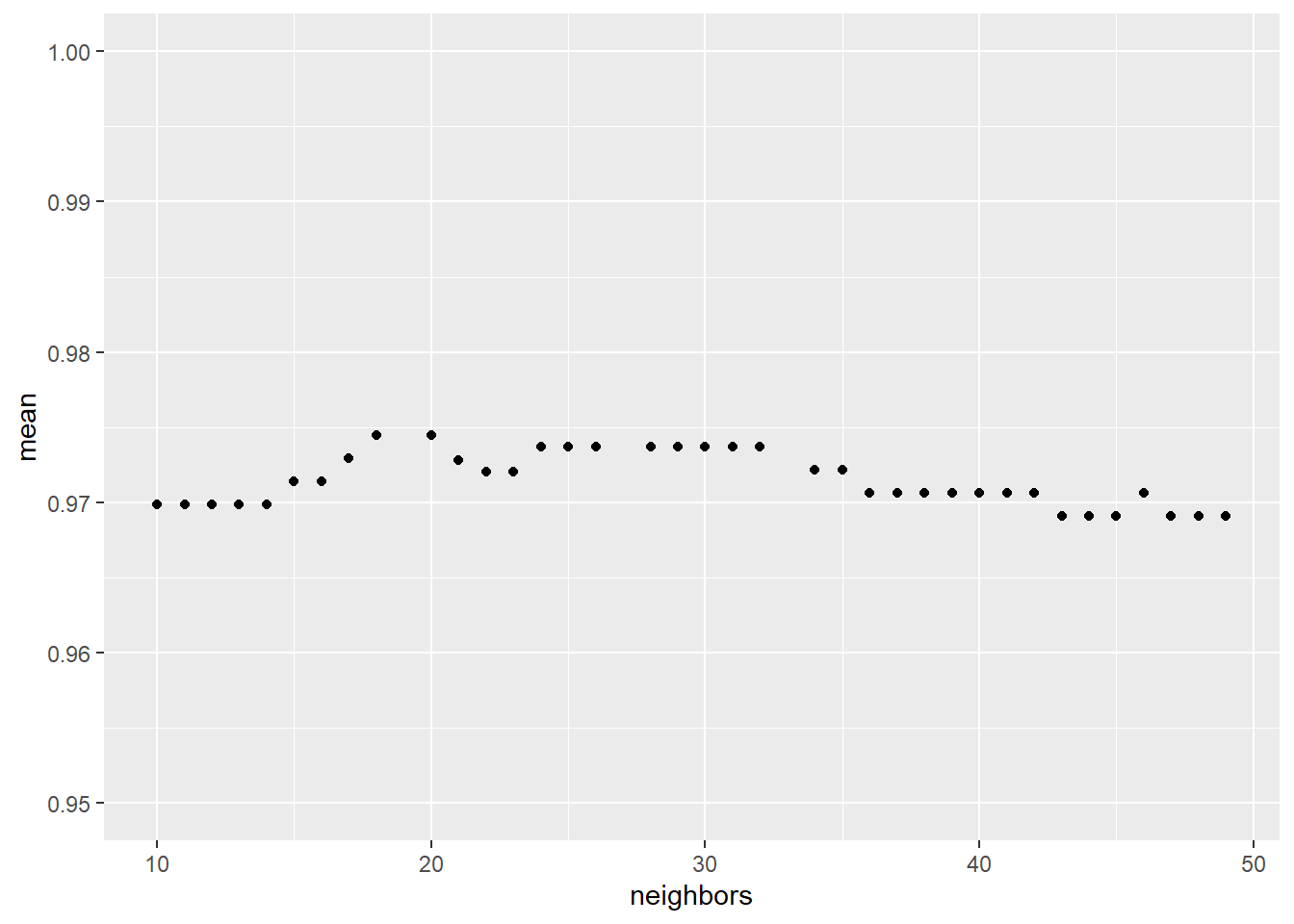 unnamed-chunk-16: 0.16 sec elapsed
Checking the timing table
(x <- tic.log() %>%
  as.character() %>%
  tibble(log = .) %>%
  separate(log,sep = ': ',into = c('name','time'))) %>%
  separate(time, sep = ' ',c('measure','units')) %>%
  mutate(measure = measure %>% as.numeric()) %>%
  arrange(measure %>% desc())
## Warning: Expected 2 pieces. Additional pieces discarded in 31 rows [1, 2, 3, 4,
## 5, 6, 7, 8, 9, 10, 11, 12, 13, 14, 15, 16, 17, 18, 19, 20, ...].## # A tibble: 31 x 3
## name measure units
## <chr> <dbl> <chr>
## 1 Bayes Search 26.4 sec
## 2 naive grid search 6.31 sec
## 3 Loading Libraries 3.65 sec
## 4 set up parallel 1.29 sec
## 5 Data Explorer individual plots 1.05 sec
## 6 Fitting production 0.28 sec
## 7 unnamed-chunk-6 0.2 sec
## 8 Set Chunk 0.16 sec
## 9 unnamed-chunk-5 0.16 sec
## 10 unnamed-chunk-16 0.16 sec
## # … with 21 more rowsunnamed-chunk-17: 0.02 sec elapsed