
- 1 Getting Started, we will use multiple functions from both languages
- 2 Python
- 2.1 Knowing data frames
- 2.2 Combining two pd series
- 2.3 Real data
- 2.3.1 Reading data
- 2.3.2 Variable types
- 2.3.3 Basic Description
- 2.3.4 Subsetting data
- 2.3.5 Creating new columns with real data
- 2.3.6 Creating a new smaller data frame
- 2.3.7 Plotting an line plot
- 2.3.8 Filtering and replace data
- 2.3.9 Groupby example
- 2.3.10 Ploting an histogram
- 2.3.11 Handling Missing values
- 2.3.12 Replacing names with an dictionary
- 2.4 Passing Objects
- 3 R
- 3.1 Knowing data frames
- 3.2 Creating an data frame from two R series
- 3.2.1 Create a date frame using an list
- 3.2.2 Create a date frame using an list 2
- 3.2.3 Subsetting an data frame using join or cbind
- 3.2.4 Some info on our data frame
- 3.2.5 Creating new columns using mutate and basic R
- 3.2.6 Ordering an data frame using the tidy way arrange or order.
- 3.2.7 Filtering rows using standard R code or filter.
- 3.3 Real Case
- 3.3.1 Two way of importing an csv
- 3.3.2 Let’s look at our data
- 3.3.3 Types of columns r
- 3.3.4 Basic Description real data using Glimpse and str
- 3.3.5 Subsetting Data with select or base R
- 3.3.6 Creating a new smaller data frame using transmute and base
- 3.3.7 Ploting with ggplot
- 3.3.8 Filtering and replace data
- 3.3.9 Groupby example in tidyverse
- 3.3.10 Ploting an histogram using ggplot2
- 3.3.11 Handling Missing values in R
- 3.3.12 Replacing names with an case when aproach
- 3.4 Passing Objects to Python
I am currently doing exercises from digital house brasil
1 Getting Started, we will use multiple functions from both languages
1.1 How to set up reticulate?
1.1.1 Setting root folder
I recommend using the Files tab to find the your system path to the folder containig all the data.
Use opts_knit to guarantee that your markdown functions will search for files in the folder specified, it is better that setwd() because it works on all languages.
knitr::opts_knit$set(root.dir = normalizePath(
  "~/R/Blog/content/post/data"))
1.1.2 Libraries

R part
library(reticulate)
library(caTools)
library(roperators)
library(tidyverse)
set.seed(123)
Python part
I am using my second virtual conda if you have just the root switch to conda_list()[[1]][1].
conda_list()[[1]][2] %>%
  use_condaenv(required = TRUE)
Let’s see what version of python this env is running.
import platform
print(platform.python_version())
## 3.7.2Some basic Data Science Libraries.
import numpy as np
import matplotlib.pyplot as plt
import pandas as pd
import os
2 Python
2.1 Knowing data frames
2.1.1 Defining pandas series

data = pd.Series([0.25, 0.5, 0.75, 1.0])
data
## 0 0.25
## 1 0.50
## 2 0.75
## 3 1.00
## dtype: float64data.values## array([0.25, 0.5 , 0.75, 1. ])data.index## RangeIndex(start=0, stop=4, step=1)data[1]## 0.5data[1:3]## 1 0.50
## 2 0.75
## dtype: float642.1.2 Indexing
data = pd.Series([0.25, 0.5, 0.75, 1.0],
                 index=['a', 'b', 'c', 'd'])
data
## a 0.25
## b 0.50
## c 0.75
## d 1.00
## dtype: float64data['b']## 0.52.2 Combining two pd series
2.2.1 Create pd series from dictionary 1
population_dict = {'California': 38332521,
                   'Florida': 19552860,
                   'Illinois': 12882135,
                   'New York': 19651127,
                   'Texas': 26448193,}
population = pd.Series(population_dict)

population
## California 38332521
## Florida 19552860
## Illinois 12882135
## New York 19651127
## Texas 26448193
## dtype: int64population['California']## 38332521population['California':'Illinois']## California 38332521
## Florida 19552860
## Illinois 12882135
## dtype: int64one more example.
area_dict = {'California': 423967,
             'Florida': 170312,
             'Illinois': 149995,
             'New York': 141297,
             'Texas': 695662}

area = pd.Series(area_dict)

area
## California 423967
## Florida 170312
## Illinois 149995
## New York 141297
## Texas 695662
## dtype: int642.2.2 Combining the pd series into a data frame
states = pd.DataFrame({'population': population,
                       'area': area})
states
## population area
## California 38332521 423967
## Florida 19552860 170312
## Illinois 12882135 149995
## New York 19651127 141297
## Texas 26448193 695662type(states)## <class 'pandas.core.frame.DataFrame'>type(states["population"])## <class 'pandas.core.series.Series'>type([states["population"]])## <class 'list'>2.2.3 Data frame properties
states.shape## (5, 2)states.info()## <class 'pandas.core.frame.DataFrame'>
## Index: 5 entries, California to Texas
## Data columns (total 2 columns):
## population 5 non-null int64
## area 5 non-null int64
## dtypes: int64(2)
## memory usage: 280.0+ bytesstates.index## Index(['California', 'Florida', 'Illinois', 'New York', 'Texas'], dtype='object')states.columns## Index(['population', 'area'], dtype='object')states['area']## California 423967
## Florida 170312
## Illinois 149995
## New York 141297
## Texas 695662
## Name: area, dtype: int642.2.4 Creating some new columns
states['density'] = states['population'] / states['area']
states
## population area density
## California 38332521 423967 90.413926
## Florida 19552860 170312 114.806121
## Illinois 12882135 149995 85.883763
## New York 19651127 141297 139.076746
## Texas 26448193 695662 38.0187402.2.5 Ordering a data frame
states.sort_values(['population'], ascending = True)## population area density
## Illinois 12882135 149995 85.883763
## Florida 19552860 170312 114.806121
## New York 19651127 141297 139.076746
## Texas 26448193 695662 38.018740
## California 38332521 423967 90.413926states.sort_values(['area'], ascending = True)## population area density
## New York 19651127 141297 139.076746
## Illinois 12882135 149995 85.883763
## Florida 19552860 170312 114.806121
## California 38332521 423967 90.413926
## Texas 26448193 695662 38.018740states.sort_values(['density'], ascending = True)## population area density
## Texas 26448193 695662 38.018740
## Illinois 12882135 149995 85.883763
## California 38332521 423967 90.413926
## Florida 19552860 170312 114.806121
## New York 19651127 141297 139.0767462.2.6 Subsetting
states['Florida':'Illinois']## population area density
## Florida 19552860 170312 114.806121
## Illinois 12882135 149995 85.883763states[1:3]## population area density
## Florida 19552860 170312 114.806121
## Illinois 12882135 149995 85.883763data_pop = (states['population'] > 19552860) & (states['area']>423967)
data_pop## California False
## Florida False
## Illinois False
## New York False
## Texas True
## dtype: boolstates[(states['population'] > 19552860) & (states['area']>423967)]## population area density
## Texas 26448193 695662 38.01874states[['area','density']]## area density
## California 423967 90.413926
## Florida 170312 114.806121
## Illinois 149995 85.883763
## New York 141297 139.076746
## Texas 695662 38.018740states[states.density > 100]## population area density
## Florida 19552860 170312 114.806121
## New York 19651127 141297 139.076746states.loc[states.density > 100, ['population', 'density']]## population density
## Florida 19552860 114.806121
## New York 19651127 139.076746states.loc[states.density > 100][['population', 'density']]## population density
## Florida 19552860 114.806121
## New York 19651127 139.076746states.loc['California', 'density']## 90.41392608386974states.loc['California'][['density']]## density 90.413926
## Name: California, dtype: float64states.iloc[0, 2]## 90.413926083869742.3 Real data
2.3.1 Reading data
sales = pd.DataFrame(pd.read_csv('2019-03-23-exploratory-data-analysis-basic-pandas-and-dplyr/UKretail.csv',encoding='latin'))sales.head()## InvoiceNo StockCode ... CustomerID Country
## 0 536365 22752 ... 17850.0 United Kingdom
## 1 536365 71053 ... 17850.0 United Kingdom
## 2 536365 84029G ... 17850.0 United Kingdom
## 3 536365 85123A ... 17850.0 United Kingdom
## 4 536366 22633 ... 17850.0 United Kingdom
##
## [5 rows x 8 columns]sales.tail(3)## InvoiceNo StockCode ... CustomerID Country
## 325142 581587 22899 ... 12680.0 France
## 325143 581587 23254 ... 12680.0 France
## 325144 581587 23256 ... 12680.0 France
##
## [3 rows x 8 columns]sales.index## RangeIndex(start=0, stop=325145, step=1)2.3.2 Variable types
If you need to return.
type(sales)
## <class 'pandas.core.frame.DataFrame'>type(sales["CustomerID"])## <class 'pandas.core.series.Series'>type([sales["CustomerID"]])
## <class 'list'>2.3.3 Basic Description
sales.shape
## (325145, 8)sales.columns.values
## array(['InvoiceNo', 'StockCode', 'Description', 'Quantity', 'InvoiceDate',
##        'UnitPrice', 'CustomerID', 'Country'], dtype=object)
sales.info()
## <class 'pandas.core.frame.DataFrame'>
## RangeIndex: 325145 entries, 0 to 325144
## Data columns (total 8 columns):
## InvoiceNo      325145 non-null object
## StockCode      325145 non-null object
## Description    324275 non-null object
## Quantity       325145 non-null int64
## InvoiceDate    325145 non-null object
## UnitPrice      325145 non-null float64
## CustomerID     244154 non-null float64
## Country        325145 non-null object
## dtypes: float64(2), int64(1), object(5)
## memory usage: 19.8+ MBsales.describe()## Quantity UnitPrice CustomerID
## count 325145.000000 325145.000000 244154.000000
## mean 9.273340 4.845239 15288.823120
## std 154.394112 116.830451 1713.496816
## min -80995.000000 -11062.060000 12347.000000
## 25% 1.000000 1.250000 13959.000000
## 50% 3.000000 2.080000 15150.000000
## 75% 10.000000 4.130000 16792.750000
## max 12540.000000 38970.000000 18287.0000002.3.4 Subsetting data
sales[:4]## InvoiceNo StockCode ... CustomerID Country
## 0 536365 22752 ... 17850.0 United Kingdom
## 1 536365 71053 ... 17850.0 United Kingdom
## 2 536365 84029G ... 17850.0 United Kingdom
## 3 536365 85123A ... 17850.0 United Kingdom
##
## [4 rows x 8 columns]sales["CustomerID"].head()## 0 17850.0
## 1 17850.0
## 2 17850.0
## 3 17850.0
## 4 17850.0
## Name: CustomerID, dtype: float64sales.loc[:,['Quantity']].head()## Quantity
## 0 2
## 1 6
## 2 6
## 3 6
## 4 6sales.iloc[:,[3]].head()## Quantity
## 0 2
## 1 6
## 2 6
## 3 6
## 4 6sales.iloc[0:6,2:3]## Description
## 0 SET 7 BABUSHKA NESTING BOXES
## 1 WHITE METAL LANTERN
## 2 KNITTED UNION FLAG HOT WATER BOTTLE
## 3 WHITE HANGING HEART T-LIGHT HOLDER
## 4 HAND WARMER UNION JACK
## 5 HOME BUILDING BLOCK WORD2.3.5 Creating new columns with real data
sales["Revenue"] = sales.Quantity * sales.UnitPricesales.head()## InvoiceNo StockCode ... Country Revenue
## 0 536365 22752 ... United Kingdom 15.30
## 1 536365 71053 ... United Kingdom 20.34
## 2 536365 84029G ... United Kingdom 20.34
## 3 536365 85123A ... United Kingdom 15.30
## 4 536366 22633 ... United Kingdom 11.10
##
## [5 rows x 9 columns]2.3.6 Creating a new smaller data frame
raw_sales = sales[["Quantity","UnitPrice", "Revenue"]]

raw_sales.head()
## Quantity UnitPrice Revenue
## 0 2 7.65 15.30
## 1 6 3.39 20.34
## 2 6 3.39 20.34
## 3 6 2.55 15.30
## 4 6 1.85 11.10raw_sales.info()## <class 'pandas.core.frame.DataFrame'>
## RangeIndex: 325145 entries, 0 to 325144
## Data columns (total 3 columns):
## Quantity 325145 non-null int64
## UnitPrice 325145 non-null float64
## Revenue 325145 non-null float64
## dtypes: float64(2), int64(1)
## memory usage: 7.4 MB2.3.7 Plotting an line plot
import matplotlib as plt
from pylab import *

sales.plot(x="InvoiceDate", y="Revenue", kind="line")

plt.show()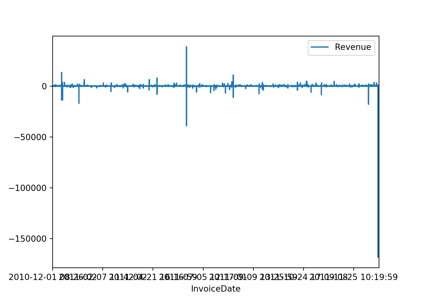
2.3.8 Filtering and replace data
To return
cancels = sales[sales["Revenue"]<0]
cancels.shape
## (5588, 9)sales.drop(cancels.index, inplace=True)
sales.shape## (319557, 9)2.3.9 Groupby example
CountryGroups = sales.groupby(["Country"])["Revenue"].sum().reset_index()
CountryGroups.sort_values(by= "Revenue", ascending=False)
## Country Revenue
## 36 United Kingdom 5311080.101
## 10 EIRE 176304.590
## 24 Netherlands 165582.790
## 14 Germany 138778.440
## 13 France 127193.680
## 0 Australia 79197.590
## 31 Spain 36116.710
## 33 Switzerland 34315.240
## 3 Belgium 24014.970
## 25 Norway 23182.220
## 32 Sweden 21762.450
## 20 Japan 21072.590
## 27 Portugal 20109.410
## 30 Singapore 13383.590
## 6 Channel Islands 12556.740
## 12 Finland 12362.880
## 9 Denmark 11739.370
## 19 Italy 10837.890
## 16 Hong Kong 8227.020
## 7 Cyprus 7781.900
## 1 Austria 6100.960
## 18 Israel 4225.780
## 26 Poland 3974.080
## 37 Unspecified 2898.650
## 15 Greece 2677.570
## 17 Iceland 2461.230
## 34 USA 2388.740
## 5 Canada 2093.390
## 23 Malta 1318.990
## 35 United Arab Emirates 1277.500
## 21 Lebanon 1120.530
## 22 Lithuania 1038.560
## 11 European Community 876.550
## 4 Brazil 602.310
## 28 RSA 573.180
## 8 Czech Republic 488.580
## 2 Bahrain 343.400
## 29 Saudi Arabia 90.7202.3.10 Ploting an histogram
sales[sales["CustomerID"] == 17850.0]["Revenue"].plot(kind="hist")
plt.show()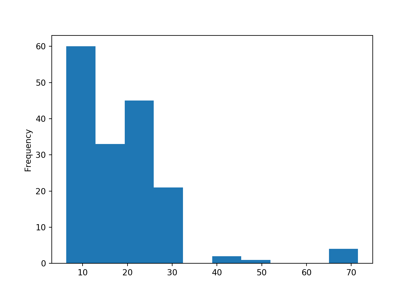
another example.
sales[sales["StockCode"] == '71053']["Quantity"].hist()
plt.show()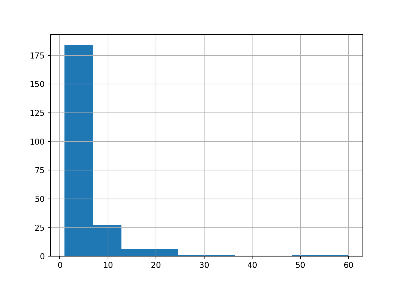
2.3.11 Handling Missing values
to return
sales.info()## <class 'pandas.core.frame.DataFrame'>
## Int64Index: 319557 entries, 0 to 325144
## Data columns (total 9 columns):
## InvoiceNo 319557 non-null object
## StockCode 319557 non-null object
## Description 318687 non-null object
## Quantity 319557 non-null int64
## InvoiceDate 319557 non-null object
## UnitPrice 319557 non-null float64
## CustomerID 238801 non-null float64
## Country 319557 non-null object
## Revenue 319557 non-null float64
## dtypes: float64(3), int64(1), object(5)
## memory usage: 24.4+ MBsales.CustomerID.value_counts(dropna=False).nlargest(3)## NaN 80756
## 17841.0 4702
## 14911.0 3449
## Name: CustomerID, dtype: int64sales.CustomerID.fillna(0, inplace=True)
sales[sales.CustomerID.isnull()]## Empty DataFrame
## Columns: [InvoiceNo, StockCode, Description, Quantity, InvoiceDate, UnitPrice, CustomerID, Country, Revenue]
## Index: []sales.info()## <class 'pandas.core.frame.DataFrame'>
## Int64Index: 319557 entries, 0 to 325144
## Data columns (total 9 columns):
## InvoiceNo 319557 non-null object
## StockCode 319557 non-null object
## Description 318687 non-null object
## Quantity 319557 non-null int64
## InvoiceDate 319557 non-null object
## UnitPrice 319557 non-null float64
## CustomerID 319557 non-null float64
## Country 319557 non-null object
## Revenue 319557 non-null float64
## dtypes: float64(3), int64(1), object(5)
## memory usage: 24.4+ MB2.3.12 Replacing names with an dictionary
mymap = {'United Kingdom':1, 'Netherlands':2, 'Germany':3, 'France':4, 'USA':5}

sales = sales.applymap(lambda s: mymap.get(s) if s in mymap else s)

sales.head()
## InvoiceNo StockCode ... Country Revenue
## 0 536365 22752 ... 1 15.30
## 1 536365 71053 ... 1 20.34
## 2 536365 84029G ... 1 20.34
## 3 536365 85123A ... 1 15.30
## 4 536366 22633 ... 1 11.10
##
## [5 rows x 9 columns]sales.Country.value_counts().nlargest(7)## 1 292640
## 3 5466
## 4 5026
## EIRE 4789
## Spain 1420
## 2 1393
## Belgium 1191
## Name: Country, dtype: int642.4 Passing Objects
2.4.1 Python to R
data2 = pd.Series([0.25, 0.5, 0.75, 1.0])data_t = py$data2data_t## 0 1 2 3
## 0.25 0.50 0.75 1.003 R
3.1 Knowing data frames
3.1.1 Defining an data frame
tidy way 
data <-  tibble(0.25, 0.5, 0.75, 1.0)
data
## # A tibble: 1 x 4
## `0.25` `0.5` `0.75` `1`
## <dbl> <dbl> <dbl> <dbl>
## 1 0.25 0.5 0.75 1data[2]## # A tibble: 1 x 1
## `0.5`
## <dbl>
## 1 0.5data[2:3]## # A tibble: 1 x 2
## `0.5` `0.75`
## <dbl> <dbl>
## 1 0.5 0.75Not using tidyverse.
data <-  data.frame(c(0.25, 0.5, 0.75, 1.0))
rownames(data) <- 1:nrow(data)
colnames(data) <- "nope"
data
## nope
## 1 0.25
## 2 0.50
## 3 0.75
## 4 1.003.1.2 Index search
data <-  data.frame(c(0.25, 0.5, 0.75, 1.0),row.names = c("a", "b","c","d"))
data
## c.0.25..0.5..0.75..1.
## a 0.25
## b 0.50
## c 0.75
## d 1.00data["b",]## [1] 0.53.2 Creating an data frame from two R series
3.2.1 Create a date frame using an list
population_dict <- list(
  'California' = 38332521,
  'Florida' = 19552860,
  'Illinois' = 12882135,
  'New York' = 19651127,
  'Texas' = 26448193
  )
population <- population_dict %>% as_tibble()

population['California']
## # A tibble: 1 x 1
## California
## <dbl>
## 1 38332521population %>% select(California:Illinois)## # A tibble: 1 x 3
## California Florida Illinois
## <dbl> <dbl> <dbl>
## 1 38332521 19552860 128821353.2.2 Create a date frame using an list 2
area_dict = list(
  'California' = 423967,
  'Florida' = 170312,
  'Illinois' = 149995,
  'New York' = 141297,
  'Texas' = 695662
  )
area_dict %>% as_tibble() -> area

area
## # A tibble: 1 x 5
## California Florida Illinois `New York` Texas
## <dbl> <dbl> <dbl> <dbl> <dbl>
## 1 423967 170312 149995 141297 6956623.2.3 Subsetting an data frame using join or cbind
The tidy way doesn`t support indexes so we can tidy our data.
tidy_area <- area %>% gather(key = "state", value = "area")
tidy_state <- population %>% gather(key = "state", value = "population")tidy_area## # A tibble: 5 x 2
## state area
## <chr> <dbl>
## 1 California 423967
## 2 Florida 170312
## 3 Illinois 149995
## 4 New York 141297
## 5 Texas 695662tidy_state## # A tibble: 5 x 2
## state population
## <chr> <dbl>
## 1 California 38332521
## 2 Florida 19552860
## 3 Illinois 12882135
## 4 New York 19651127
## 5 Texas 26448193tidy_area %>% left_join(tidy_state)## Joining, by = "state"## # A tibble: 5 x 3
## state area population
## <chr> <dbl> <dbl>
## 1 California 423967 38332521
## 2 Florida 170312 19552860
## 3 Illinois 149995 12882135
## 4 New York 141297 19651127
## 5 Texas 695662 26448193tidy_merge <- cbind(tidy_area,tidy_state[,-1])
states <- tidy_merge3.2.4 Some info on our data frame
class(tidy_merge)## [1] "data.frame"class(tidy_merge$population)## [1] "numeric"class(list(tidy_merge["population"]))## [1] "list"states %>% dim()## [1] 5 3states %>% str()## 'data.frame': 5 obs. of 3 variables:
## $ state : chr "California" "Florida" "Illinois" "New York" ...
## $ area : num 423967 170312 149995 141297 695662
## $ population: num 38332521 19552860 12882135 19651127 26448193states %>% glimpse()## Observations: 5
## Variables: 3
## $ state <chr> "California", "Florida", "Illinois", "New York", "T...
## $ area <dbl> 423967, 170312, 149995, 141297, 695662
## $ population <dbl> 38332521, 19552860, 12882135, 19651127, 26448193states[["Estado"]]## NULLstates %>% colnames() %>% tail(-1)## [1] "area" "population"states$area## [1] 423967 170312 149995 141297 6956623.2.5 Creating new columns using mutate and basic R
states$density <-  states$population / states$area
states
## state area population density
## 1 California 423967 38332521 90.41393
## 2 Florida 170312 19552860 114.80612
## 3 Illinois 149995 12882135 85.88376
## 4 New York 141297 19651127 139.07675
## 5 Texas 695662 26448193 38.01874# or
states$density <- states[["population"]] / states[["area"]]
states## state area population density
## 1 California 423967 38332521 90.41393
## 2 Florida 170312 19552860 114.80612
## 3 Illinois 149995 12882135 85.88376
## 4 New York 141297 19651127 139.07675
## 5 Texas 695662 26448193 38.01874#or
states %>%
mutate(density = population / area)## state area population density
## 1 California 423967 38332521 90.41393
## 2 Florida 170312 19552860 114.80612
## 3 Illinois 149995 12882135 85.88376
## 4 New York 141297 19651127 139.07675
## 5 Texas 695662 26448193 38.018743.2.6 Ordering an data frame using the tidy way arrange or order.
You can also use -c() or desc() sometimes -c() can give strange results.
states %>% arrange(desc(population))## state area population density
## 1 California 423967 38332521 90.41393
## 2 Texas 695662 26448193 38.01874
## 3 New York 141297 19651127 139.07675
## 4 Florida 170312 19552860 114.80612
## 5 Illinois 149995 12882135 85.88376states[order(states$area),]## state area population density
## 4 New York 141297 19651127 139.07675
## 3 Illinois 149995 12882135 85.88376
## 2 Florida 170312 19552860 114.80612
## 1 California 423967 38332521 90.41393
## 5 Texas 695662 26448193 38.01874# Mix and match all three formas
states %>% arrange(-c(density),desc(population,area),state)## state area population density
## 1 New York 141297 19651127 139.07675
## 2 Florida 170312 19552860 114.80612
## 3 California 423967 38332521 90.41393
## 4 Illinois 149995 12882135 85.88376
## 5 Texas 695662 26448193 38.018743.2.7 Filtering rows using standard R code or filter.
states[1:3,]## state area population density
## 1 California 423967 38332521 90.41393
## 2 Florida 170312 19552860 114.80612
## 3 Illinois 149995 12882135 85.88376data_pop <- states[states$population > 19552860 & states$area > 423967,]
data_pop## state area population density
## 5 Texas 695662 26448193 38.01874states %>%
filter(population > 19552860 & area > 423967)## state area population density
## 1 Texas 695662 26448193 38.01874you can mix and match filter for rows and select for columns.
states %>%
  filter(density > 100)
## state area population density
## 1 Florida 170312 19552860 114.8061
## 2 New York 141297 19651127 139.0767states %>%
filter(density > 100) %>%
select(population,density)## population density
## 1 19552860 114.8061
## 2 19651127 139.0767states[1,4]## [1] 90.413933.3 Real Case
3.3.1 Two way of importing an csv
sales <- read_csv('2019-03-23-exploratory-data-analysis-basic-pandas-and-dplyr/UKretail.csv')## Parsed with column specification:
## cols(
## InvoiceNo = col_character(),
## StockCode = col_character(),
## Description = col_character(),
## Quantity = col_double(),
## InvoiceDate = col_datetime(format = ""),
## UnitPrice = col_double(),
## CustomerID = col_double(),
## Country = col_character()
## )sales <- read.csv('2019-03-23-exploratory-data-analysis-basic-pandas-and-dplyr/UKretail.csv')If you think this looks like an ugly path and a was of space I would agree we
can fix this by using one of my favorite thinks from python the ""key I avoided.
I am now using it on the python part to show the power of neat line.
path_file = '\
2019-03-23-exploratory-data-analysis-basic-pandas-and-dplyr/\
UKretail.csv'
sales <- read_csv(py$path_file)## Parsed with column specification:
## cols(
## InvoiceNo = col_character(),
## StockCode = col_character(),
## Description = col_character(),
## Quantity = col_double(),
## InvoiceDate = col_datetime(format = ""),
## UnitPrice = col_double(),
## CustomerID = col_double(),
## Country = col_character()
## )Finally our first usefull python to r functionality!
3.3.2 Let’s look at our data
sales %>% head()## # A tibble: 6 x 8
## InvoiceNo StockCode Description Quantity InvoiceDate UnitPrice
## <chr> <chr> <chr> <dbl> <dttm> <dbl>
## 1 536365 22752 SET 7 BABU~ 2 2010-12-01 08:26:02 7.65
## 2 536365 71053 WHITE META~ 6 2010-12-01 08:26:02 3.39
## 3 536365 84029G KNITTED UN~ 6 2010-12-01 08:26:02 3.39
## 4 536365 85123A WHITE HANG~ 6 2010-12-01 08:26:02 2.55
## 5 536366 22633 HAND WARME~ 6 2010-12-01 08:28:02 1.85
## 6 536367 21754 HOME BUILD~ 3 2010-12-01 08:33:59 5.95
## # ... with 2 more variables: CustomerID <dbl>, Country <chr>sales %>% tail(3)## # A tibble: 3 x 8
## InvoiceNo StockCode Description Quantity InvoiceDate UnitPrice
## <chr> <chr> <chr> <dbl> <dttm> <dbl>
## 1 581587 22899 CHILDREN'S~ 6 2011-12-09 12:49:59 2.1
## 2 581587 23254 CHILDRENS ~ 4 2011-12-09 12:49:59 4.15
## 3 581587 23256 CHILDRENS ~ 4 2011-12-09 12:49:59 4.15
## # ... with 2 more variables: CustomerID <dbl>, Country <chr>3.3.3 Types of columns r
If you payed attention read_ tries to inform what conversion was used in each column that is specially cool because base R tends to create unesceassary factor whne in fact you are working with strings, but know you can choose between three different implementation of the read command.
A cool thing about tibbles is that they are in fact still data.frame.
sales %>% class()## [1] "spec_tbl_df" "tbl_df" "tbl" "data.frame"Pay attention to the R difference between “[[” and “[” if you recall this is the “opposite” of the python behavior.
Jump to python implementation.
sales[["CustomerID"]] %>% class()## [1] "numeric"sales["CustomerID"] %>% class()## [1] "tbl_df" "tbl" "data.frame"3.3.4 Basic Description real data using Glimpse and str
sales %>% dim()## [1] 325145 8sales %>% colnames()## [1] "InvoiceNo" "StockCode" "Description" "Quantity" "InvoiceDate"
## [6] "UnitPrice" "CustomerID" "Country"sales %>% glimpse()## Observations: 325,145
## Variables: 8
## $ InvoiceNo <chr> "536365", "536365", "536365", "536365", "536366", ...
## $ StockCode <chr> "22752", "71053", "84029G", "85123A", "22633", "21...
## $ Description <chr> "SET 7 BABUSHKA NESTING BOXES", "WHITE METAL LANTE...
## $ Quantity <dbl> 2, 6, 6, 6, 6, 3, 3, 4, 6, 6, 6, 8, 4, 3, 3, 48, 2...
## $ InvoiceDate <dttm> 2010-12-01 08:26:02, 2010-12-01 08:26:02, 2010-12...
## $ UnitPrice <dbl> 7.65, 3.39, 3.39, 2.55, 1.85, 5.95, 5.95, 7.95, 1....
## $ CustomerID <dbl> 17850, 17850, 17850, 17850, 17850, 13047, 13047, 1...
## $ Country <chr> "United Kingdom", "United Kingdom", "United Kingdo...sales %>% str()## Classes 'spec_tbl_df', 'tbl_df', 'tbl' and 'data.frame': 325145 obs. of 8 variables:
## $ InvoiceNo : chr "536365" "536365" "536365" "536365" ...
## $ StockCode : chr "22752" "71053" "84029G" "85123A" ...
## $ Description: chr "SET 7 BABUSHKA NESTING BOXES" "WHITE METAL LANTERN" "KNITTED UNION FLAG HOT WATER BOTTLE" "WHITE HANGING HEART T-LIGHT HOLDER" ...
## $ Quantity : num 2 6 6 6 6 3 3 4 6 6 ...
## $ InvoiceDate: POSIXct, format: "2010-12-01 08:26:02" "2010-12-01 08:26:02" ...
## $ UnitPrice : num 7.65 3.39 3.39 2.55 1.85 5.95 5.95 7.95 1.65 2.1 ...
## $ CustomerID : num 17850 17850 17850 17850 17850 ...
## $ Country : chr "United Kingdom" "United Kingdom" "United Kingdom" "United Kingdom" ...
## - attr(*, "spec")=
## .. cols(
## .. InvoiceNo = col_character(),
## .. StockCode = col_character(),
## .. Description = col_character(),
## .. Quantity = col_double(),
## .. InvoiceDate = col_datetime(format = ""),
## .. UnitPrice = col_double(),
## .. CustomerID = col_double(),
## .. Country = col_character()
## .. )sales %>% summary()## InvoiceNo StockCode Description
## Length:325145 Length:325145 Length:325145
## Class :character Class :character Class :character
## Mode :character Mode :character Mode :character
##
##
##
##
## Quantity InvoiceDate UnitPrice
## Min. :-80995.00 Min. :2010-12-01 08:26:02 Min. :-11062.06
## 1st Qu.: 1.00 1st Qu.:2011-03-28 12:13:02 1st Qu.: 1.25
## Median : 3.00 Median :2011-07-20 10:50:59 Median : 2.08
## Mean : 9.27 Mean :2011-07-04 14:11:43 Mean : 4.85
## 3rd Qu.: 10.00 3rd Qu.:2011-10-19 10:47:59 3rd Qu.: 4.13
## Max. : 12540.00 Max. :2011-12-09 12:49:59 Max. : 38970.00
##
## CustomerID Country
## Min. :12347 Length:325145
## 1st Qu.:13959 Class :character
## Median :15150 Mode :character
## Mean :15289
## 3rd Qu.:16793
## Max. :18287
## NA's :80991If you agree with me that summary sucks on a data.frame object I am glad to show skimr, also if you don’t like summary behaviour on model outputs broom is there to save you, I will talk more about when I make an scikit-learn and caret + tidymodels post.
3.3.5 Subsetting Data with select or base R
sales[1:4,]## # A tibble: 4 x 8
## InvoiceNo StockCode Description Quantity InvoiceDate UnitPrice
## <chr> <chr> <chr> <dbl> <dttm> <dbl>
## 1 536365 22752 SET 7 BABU~ 2 2010-12-01 08:26:02 7.65
## 2 536365 71053 WHITE META~ 6 2010-12-01 08:26:02 3.39
## 3 536365 84029G KNITTED UN~ 6 2010-12-01 08:26:02 3.39
## 4 536365 85123A WHITE HANG~ 6 2010-12-01 08:26:02 2.55
## # ... with 2 more variables: CustomerID <dbl>, Country <chr>sales$CustomerID %>% head()## [1] 17850 17850 17850 17850 17850 13047sales[["CustomerID"]] %>% head()## [1] 17850 17850 17850 17850 17850 13047sales[,3] %>% head()## # A tibble: 6 x 1
## Description
## <chr>
## 1 SET 7 BABUSHKA NESTING BOXES
## 2 WHITE METAL LANTERN
## 3 KNITTED UNION FLAG HOT WATER BOTTLE
## 4 WHITE HANGING HEART T-LIGHT HOLDER
## 5 HAND WARMER UNION JACK
## 6 HOME BUILDING BLOCK WORDsales[1:5,3]## # A tibble: 5 x 1
## Description
## <chr>
## 1 SET 7 BABUSHKA NESTING BOXES
## 2 WHITE METAL LANTERN
## 3 KNITTED UNION FLAG HOT WATER BOTTLE
## 4 WHITE HANGING HEART T-LIGHT HOLDER
## 5 HAND WARMER UNION JACKsales$Revenue2 <- sales$Quantity * sales$UnitPrice
sales[["Revenue3"]] <- sales[["Quantity"]] * sales[["UnitPrice"]]
# () show created objects
# Strange behavior right here 6 rowns on head()
(sales <- sales %>% mutate(Revenue = Quantity * UnitPrice)) %>% head()## # A tibble: 6 x 11
## InvoiceNo StockCode Description Quantity InvoiceDate UnitPrice
## <chr> <chr> <chr> <dbl> <dttm> <dbl>
## 1 536365 22752 SET 7 BABU~ 2 2010-12-01 08:26:02 7.65
## 2 536365 71053 WHITE META~ 6 2010-12-01 08:26:02 3.39
## 3 536365 84029G KNITTED UN~ 6 2010-12-01 08:26:02 3.39
## 4 536365 85123A WHITE HANG~ 6 2010-12-01 08:26:02 2.55
## 5 536366 22633 HAND WARME~ 6 2010-12-01 08:28:02 1.85
## 6 536367 21754 HOME BUILD~ 3 2010-12-01 08:33:59 5.95
## # ... with 5 more variables: CustomerID <dbl>, Country <chr>,
## # Revenue2 <dbl>, Revenue3 <dbl>, Revenue <dbl>sum(sales$Revenue == sales$Revenue2)/nrow(sales)## [1] 1sum(sales$Revenue == sales$Revenue3)/nrow(sales)## [1] 1sum(sales$Revenue2 == sales$Revenue3)/nrow(sales)## [1] 1# If there were any differences between our columns the sum would return <1 3.3.6 Creating a new smaller data frame using transmute and base
raw_sales <- sales %>% select(Quantity, UnitPrice, Revenue)

raw_sales %>% head()
## # A tibble: 6 x 3
## Quantity UnitPrice Revenue
## <dbl> <dbl> <dbl>
## 1 2 7.65 15.3
## 2 6 3.39 20.3
## 3 6 3.39 20.3
## 4 6 2.55 15.3
## 5 6 1.85 11.1
## 6 3 5.95 17.8raw_sales %>% glimpse()## Observations: 325,145
## Variables: 3
## $ Quantity <dbl> 2, 6, 6, 6, 6, 3, 3, 4, 6, 6, 6, 8, 4, 3, 3, 48, 24,...
## $ UnitPrice <dbl> 7.65, 3.39, 3.39, 2.55, 1.85, 5.95, 5.95, 7.95, 1.65...
## $ Revenue <dbl> 15.30, 20.34, 20.34, 15.30, 11.10, 17.85, 17.85, 31....raw_sales %>% skimr::skim()## Skim summary statistics
## n obs: 325145
## n variables: 3
##
## -- Variable type:numeric ------------------------------------------------
## variable missing complete n mean sd p0 p25 p50 p75
## Quantity 0 325145 325145 9.27 154.39 -80995 1 3 10
## Revenue 0 325145 325145 17.43 331.85 -168469.6 3.4 9.48 17.4
## UnitPrice 0 325145 325145 4.85 116.83 -11062.06 1.25 2.08 4.13
## p100 hist
## 12540 <U+2581><U+2581><U+2581><U+2581><U+2581><U+2581><U+2587><U+2581>
## 38970 <U+2581><U+2581><U+2581><U+2581><U+2581><U+2581><U+2587><U+2581>
## 38970 <U+2581><U+2587><U+2581><U+2581><U+2581><U+2581><U+2581><U+2581>3.3.7 Ploting with ggplot
sales %>% ggplot() +
  aes(x = InvoiceDate, y = Revenue) +
  geom_line()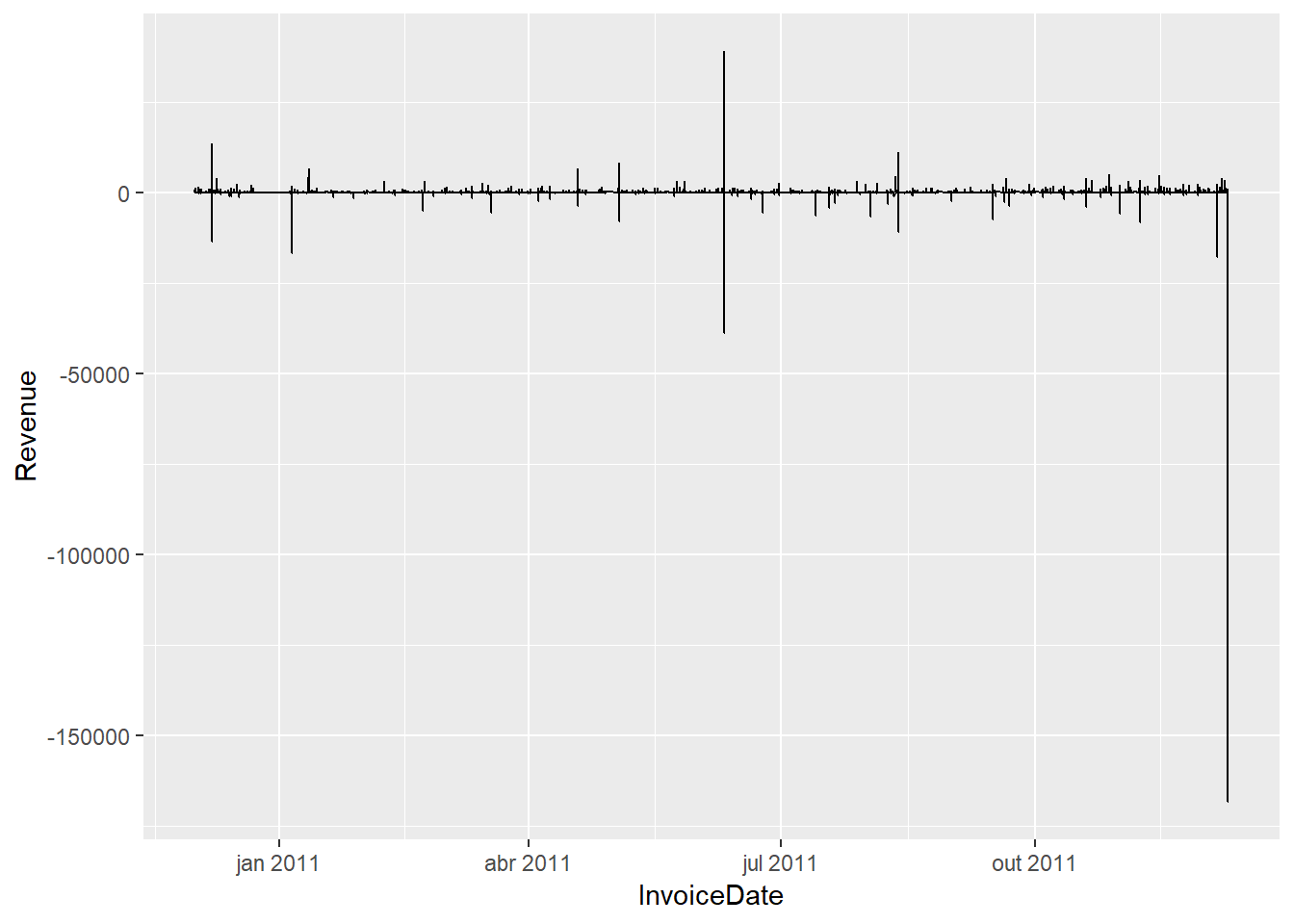
3.3.8 Filtering and replace data
Here I really couldn`t figure out an easy way to filter using this cancel tricky that works in python.
cancels = sales$Revenue < 0
cancels %>% nrow()
## NULLinvert_func <- function(cancel){
ifelse(cancel == 1,
0,
1)
}
sales2 = sales[invert_func(cancels),]
sales2 %>% dim()## [1] 319557 11I really prefer the tidy way also.
sales <- sales %>% filter(Revenue > 0)3.3.9 Groupby example in tidyverse
I prefer the tidy way here as well.
CountryGroups <- sales %>%
  group_by(Country) %>%
  summarise(sum_revenue = sum(Revenue),
            number_cases = n()) %>%
  arrange(-sum_revenue)

CountryGroups
## # A tibble: 38 x 3
## Country sum_revenue number_cases
## <chr> <dbl> <int>
## 1 United Kingdom 5311080. 291129
## 2 EIRE 176305. 4788
## 3 Netherlands 165583. 1391
## 4 Germany 138778. 5465
## 5 France 127194. 5025
## 6 Australia 79198. 726
## 7 Spain 36117. 1420
## 8 Switzerland 34315. 1169
## 9 Belgium 24015. 1191
## 10 Norway 23182. 658
## # ... with 28 more rowsskimr::skim(sales)## Skim summary statistics
## n obs: 318036
## n variables: 11
##
## -- Variable type:character ----------------------------------------------
## variable missing complete n min max empty n_unique
## Country 0 318036 318036 3 20 0 38
## Description 0 318036 318036 6 35 0 3926
## InvoiceNo 0 318036 318036 6 7 0 19107
## StockCode 0 318036 318036 1 12 0 3835
##
## -- Variable type:numeric ------------------------------------------------
## variable missing complete n mean sd p0 p25
## CustomerID 79261 238775 318036 15295.34 1713.1 12347 13969
## Quantity 0 318036 318036 10.25 38.3 1 1
## Revenue 0 318036 318036 19.78 104.17 0.001 3.75
## Revenue2 0 318036 318036 19.78 104.17 0.001 3.75
## Revenue3 0 318036 318036 19.78 104.17 0.001 3.75
## UnitPrice 0 318036 318036 3.96 42.53 0.001 1.25
## p50 p75 p100 hist
## 15157 16800 18287 <U+2587><U+2586><U+2587><U+2587><U+2586><U+2586><U+2586><U+2587>
## 3 10 4800 <U+2587><U+2581><U+2581><U+2581><U+2581><U+2581><U+2581><U+2581>
## 9.9 17.7 38970 <U+2587><U+2581><U+2581><U+2581><U+2581><U+2581><U+2581><U+2581>
## 9.9 17.7 38970 <U+2587><U+2581><U+2581><U+2581><U+2581><U+2581><U+2581><U+2581>
## 9.9 17.7 38970 <U+2587><U+2581><U+2581><U+2581><U+2581><U+2581><U+2581><U+2581>
## 2.08 4.13 13541.33 <U+2587><U+2581><U+2581><U+2581><U+2581><U+2581><U+2581><U+2581>
##
## -- Variable type:POSIXct ------------------------------------------------
## variable missing complete n min max median
## InvoiceDate 0 318036 318036 2010-12-01 2011-12-09 2011-07-20
## n_unique
## 177503.3.10 Ploting an histogram using ggplot2
sales %>%
  filter(CustomerID == 17850) %>%
  ggplot() +
  aes(Revenue) +
  geom_histogram(bins = 20)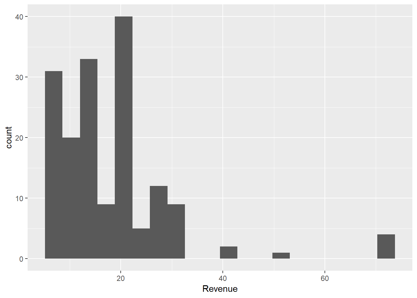
Another example.
sales %>%
  filter(StockCode == 71053) %>%
  ggplot() +
  aes(Revenue) +
  geom_histogram(bins = 20)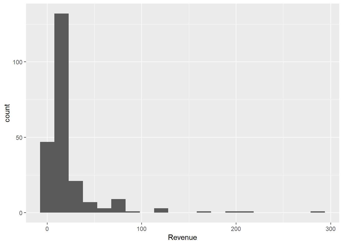
3.3.11 Handling Missing values in R
Ok I got hand this one to python.
sales2$CustomerID %>%
  table(useNA = 'always') %>%
  sort(decreasing = TRUE) %>%
  head(3)
## .
## 17850 <NA>
## 319557 0This is just not simple enough luckly we can create functions for our afflictions, plus this is replacement as an side effect which sucks.
#sales[sales[["CustomerID"]] %>% is.na(),"CustomerID"] <- 0This is an way better tidy way.
# sales %>% mutate_if(is.numeric, funs(replace(., is.na(.), 0)))
sales2 <- sales %>% mutate_at(vars(CustomerID),
                    list(
                      ~replace(.,
                              is.na(.), # function that check condition (na)
                              0) # value to replace could be mean(.,na.rm = T)
                      )
                    )
Using an stronger method like mice even with an amazing multicore package takes too long for an blogpost, plus I really don’t think there should be an model for CustomerID here is some workflow if you need to split your data.
non_character_sales <- sales %>%
  select_if(function(col)
    is.numeric(col) |
      is.factor(col))

# or my favorite
select_cases <- function(col) {
  is.numeric(col) |
  is.factor(col)
}

non_character_sales <- sales %>% select_if(select_cases)

non_character_sales %>% head()
## # A tibble: 6 x 6
## Quantity UnitPrice CustomerID Revenue2 Revenue3 Revenue
## <dbl> <dbl> <dbl> <dbl> <dbl> <dbl>
## 1 2 7.65 17850 15.3 15.3 15.3
## 2 6 3.39 17850 20.3 20.3 20.3
## 3 6 3.39 17850 20.3 20.3 20.3
## 4 6 2.55 17850 15.3 15.3 15.3
## 5 6 1.85 17850 11.1 11.1 11.1
## 6 3 5.95 13047 17.8 17.8 17.8character_sales <- sales %>% select_if(negate(is.numeric))
character_sales %>% head()## # A tibble: 6 x 5
## InvoiceNo StockCode Description InvoiceDate Country
## <chr> <chr> <chr> <dttm> <chr>
## 1 536365 22752 SET 7 BABUSHKA NESTIN~ 2010-12-01 08:26:02 United Ki~
## 2 536365 71053 WHITE METAL LANTERN 2010-12-01 08:26:02 United Ki~
## 3 536365 84029G KNITTED UNION FLAG HO~ 2010-12-01 08:26:02 United Ki~
## 4 536365 85123A WHITE HANGING HEART T~ 2010-12-01 08:26:02 United Ki~
## 5 536366 22633 HAND WARMER UNION JACK 2010-12-01 08:28:02 United Ki~
## 6 536367 21754 HOME BUILDING BLOCK W~ 2010-12-01 08:33:59 United Ki~sales3 <- cbind(character_sales,non_character_sales)
# if you need the same order
sales3 <- sales3 %>% select(names(sales)) 3.3.12 Replacing names with an case when aproach
Don’t mix and match numbers and characters else this will cause an error.
replace_function <-  function(country) {
  case_when(
  country == 'United Kingdom' ~ "1",
  country == 'Netherlands' ~ "2",
  country == 'Germany' ~ "3",
  country == 'France' ~ "4",
  country == 'USA' ~ "5",
  TRUE    ~ country
)
  }
sales3 <- sales3 %>% mutate(new = replace_function(Country))
sales3 %>% head()## InvoiceNo StockCode Description Quantity
## 1 536365 22752 SET 7 BABUSHKA NESTING BOXES 2
## 2 536365 71053 WHITE METAL LANTERN 6
## 3 536365 84029G KNITTED UNION FLAG HOT WATER BOTTLE 6
## 4 536365 85123A WHITE HANGING HEART T-LIGHT HOLDER 6
## 5 536366 22633 HAND WARMER UNION JACK 6
## 6 536367 21754 HOME BUILDING BLOCK WORD 3
## InvoiceDate UnitPrice CustomerID Country Revenue2
## 1 2010-12-01 08:26:02 7.65 17850 United Kingdom 15.30
## 2 2010-12-01 08:26:02 3.39 17850 United Kingdom 20.34
## 3 2010-12-01 08:26:02 3.39 17850 United Kingdom 20.34
## 4 2010-12-01 08:26:02 2.55 17850 United Kingdom 15.30
## 5 2010-12-01 08:28:02 1.85 17850 United Kingdom 11.10
## 6 2010-12-01 08:33:59 5.95 13047 United Kingdom 17.85
## Revenue3 Revenue new
## 1 15.30 15.30 1
## 2 20.34 20.34 1
## 3 20.34 20.34 1
## 4 15.30 15.30 1
## 5 11.10 11.10 1
## 6 17.85 17.85 1Two ways of solving our case_count deficiency.
value_counts <- function(column, useNA = 'always', decreasing = TRUE) {
  column %>%
  table(useNA = useNA) %>%
  sort(decreasing = decreasing)
}

sales3[["new"]] %>% value_counts() %>% head(7)
## .
## 1 3 4 EIRE Spain 2 Belgium
## 291129 5465 5025 4788 1420 1391 11913.4 Passing Objects to Python
Simple example.
sales2 = r.sales2
type(sales2)
## <class 'pandas.core.frame.DataFrame'>We can solve our value_counts problem by simply stealing from python then returning the results to r.
sales3_solution = \
r.\
sales3.\
new.\
value_counts().\
nlargest(7)
If we want to continue working in r after the steal.
sales3_solution = py$sales3_solution
sales3_solution
## 1 3 4 EIRE Spain 2 Belgium
## 291129 5465 5025 4788 1420 1391 1191